Gimond's stuff

You can download data for this example here.

year = 2010
city = "Waterville"
seas.tmp  = c("4-01", "7-01", "10-01", "12-31")
seas = as.Date(paste(seas.tmp, toString(year), sep = "-"),
format = "%m-%d-%Y", tz = "EST")

# Load data and convert date field to a date (POSIX) object.
# The date/time is in standard time.
met.raw  = read.csv ( paste(city, "_", toString(year), 
           ".csv", sep = ""),
            na.strings = c("NaN", "M"),header = T ) 
met.day = as.Date(met.raw$Date,
          format="%m/%d/%Y", tz="EST") # extract date/time column. No DST.
met.1 = met.raw[, -2]
met   = data.frame(Date = met.day,met.1)
# column to met.1 (overwrite met object)
days.un = unique(met$Date)
day.mean = tapply(met$Temp, met$Date, median, na.rm = T)
day.hdd  = data.frame(Date = days.un, HDD = (65-day.mean), 
            IO=((65 - day.mean) > 0))

day.hdd.sub1 = subset(day.hdd, HDD > 0) # Only positive HDD values are used
csum.tmp  =  cumsum(day.hdd.sub1$HDD)
day.hdd.csum = data.frame(Date = day.hdd.sub1$Date,
               HDD.CD = csum.tmp, IO = day.hdd.sub1$IO)

# Find the cumulative HDD for the end of each season
seas.df    = data.frame(eDate = seas)
seas.index = findInterval(seas, day.hdd.csum$Date) # Find the closest date
hdd.seas   = day.hdd.csum[seas.index,]             # Cumulative HDD by season

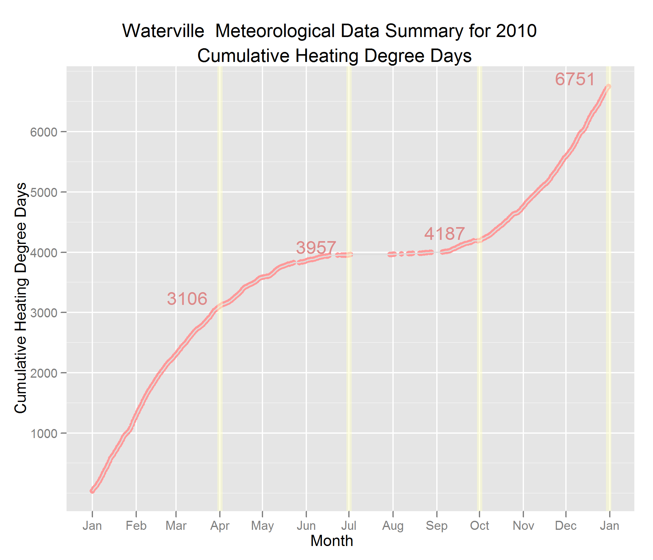
p  <- ggplot(day.hdd.csum, aes(Date, HDD.CD) )
p2 <- p + geom_point(aes(colour = IO))                     +
      scale_colour_manual(values = c("#ff9999"))           +
      scale_x_date("Month", format = "%b",
      major = "months", minor = "months")                  +
      scale_y_continuous("Cumulative Heating Degree Days") +
      geom_line(aes(Date, HDD.CD), colour = "#dddddd")     +
      geom_vline(aes(xintercept = eDate),data=seas.df,
      colour="#ffffcc", alpha = I(1/2),
      size = 2)                                            +
      geom_text(aes(x = Date, label = as.integer(HDD.CD),
      hjust = 1.3,vjust = -0.1), data = hdd.seas,
      colour="#dd8888")                                    +
      opts(legend.position = "none",
      title = paste(city," Meteorological Data Summary for",
      year, "\n Cumulative Heating Degree Days"))

ggsave(paste(city, "_", year, "_HDD.png", sep = ""), plot = p2,
width = 7, height = 6)