Gimond's stuff

!! Data for this exercise can be downloaded from here !!

library(maptools)

S = readShapePoints("points_krig.shp")

#Convert data to spatstat format
SP  = as(S, "SpatialPoints")# This only grabs the X,Y values
SPz = slot(S,"data") # This grabs all attribute values
P   = as(SP, "ppp") # This creates a spatstat point pattern
marks(P) = SPz # This add the attribute values to P
#
# thus creating a marked point pattern
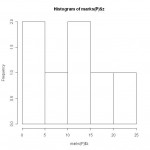
hist(marks(P)$z) # plots histogram of attribute z

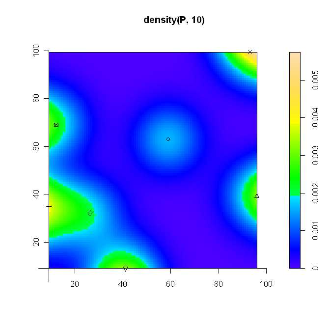
# Convert data to dataframe
P.frame = as.data.frame(P)
# Only keep necessary columns
P.frame.sub = data.frame(x=P.frame$x,y=P.frame$y,z=P.frame$z)
#
# Get individual columns
X = P.frame$x
Y = P.frame$y
Z = P.frame$z
#
# Check plot (note the bullseye effect of the standard interpolation)
plot(density(P,10),axes=T)
plot(P, add=T)

# Use geoR package
# Create a trend surface
library(geoR)
P.cloud=variog(coords = cbind(X,Y), data=Z, option=c("cloud"))
plot(P.cloud)

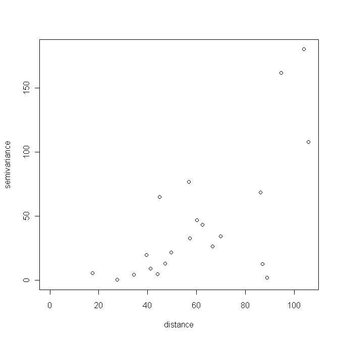
P.bin = variog(coords = cbind(X,Y), data=Z, uvec=seq(0,100,l=10))
plot(P.bin)

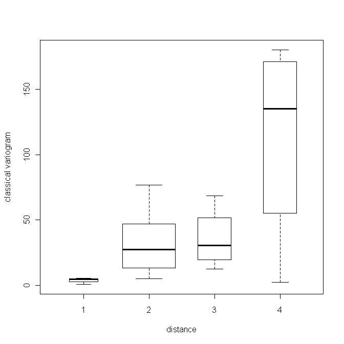
#Bins can be displayed with a box-plot for each bin
P.bin1 = variog(coords = cbind(X,Y), data=Z, uvec=seq(0,100,l=5), bin.cloud = T)
plot(P.bin1, bin.cloud=T,main="Classical estimator")

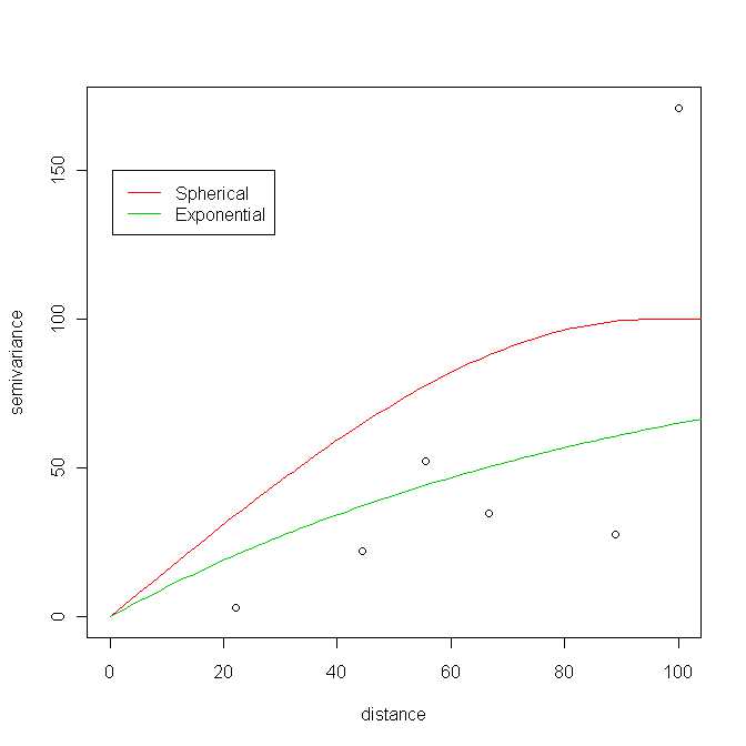
# Theoretical and empirical variograms can be plotted and visually compared
plot(P.bin)
lines.variomodel(cov.model= "spherical", cov.pars = c(100,95), 
                 nugget = 0, max.dist=120,lwd=1, col=2)
lines.variomodel(cov.model= "exponential", cov.pars = c(100,95), 
                 nugget = 0, max.dist=120,lwd=1, col=3)

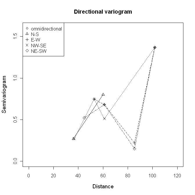
# computing a directional variogram
plot(0,0,xlab="Distance",ylab="Semivariogram",xlim=c(0,120),ylim=c(0,1.6),cex.lab=1.2,type="n")
title("Directional variogram",cex.main=1.2)
lines(P.bin,pch=1,type="p")
vario.0 = variog(coords=cbind(X,Y), data=Z, lambda=0, max.dist=120, dir=0, tol=pi/4)
vario.90 = variog(coords=cbind(X,Y), data=Z, lambda=0, max.dist=120, dir=pi/4, tol=pi/4)
vario.45 = variog(coords=cbind(X,Y), data=Z, lambda=0, max.dist=120, dir=pi/8, tol=pi/4)
vario.120 = variog(coords=cbind(X,Y), data=Z, lambda=0, max.dist=120, dir=3*pi/8, tol=pi/4)
lines(vario.0,lty=1,pch=2)
lines(vario.90,lty=2,pch=3)
lines(vario.45,lty=3,pch=4)
lines(vario.120,lty=4,pch=5)
legend("topleft", legend=c("omnidirectional","N-S","E-W","NW-SE","NE-SW"), pch=c(1,2,3,4,5))
#
# NOTE: pair distances are stored in P.cloud$u (P.cloud is a variogram class)

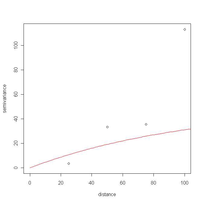
# Using the maximum likelihood technique
# Nugget fit to 0, sill=100, range=95
ml = likfit(coord=cbind(X,Y),data=Z, ini = c(100,95), fix.nugget = T) 
plot(P.bin1)
lines(ml,col=2)

# Predict a single value
plot(cbind(X,Y), xlim=c(0,100), ylim=c(0,100), xlab="Coord X", ylab="Coord Y")
loci =matrix(c(50,50),ncol=2)
text(loci, as.character(1), col="red")
kc4 = krige.conv(coord=cbind(X,Y),data=Z, locations = loci, krige = krige.control(obj.m = ml))

> kc4$predict
     data
      10.74597
      data 10.74597
# kc4$predict is the predicted value (e.g. 10.7) and 
# kc4$krige.var is the variance (e.g. 9.4)

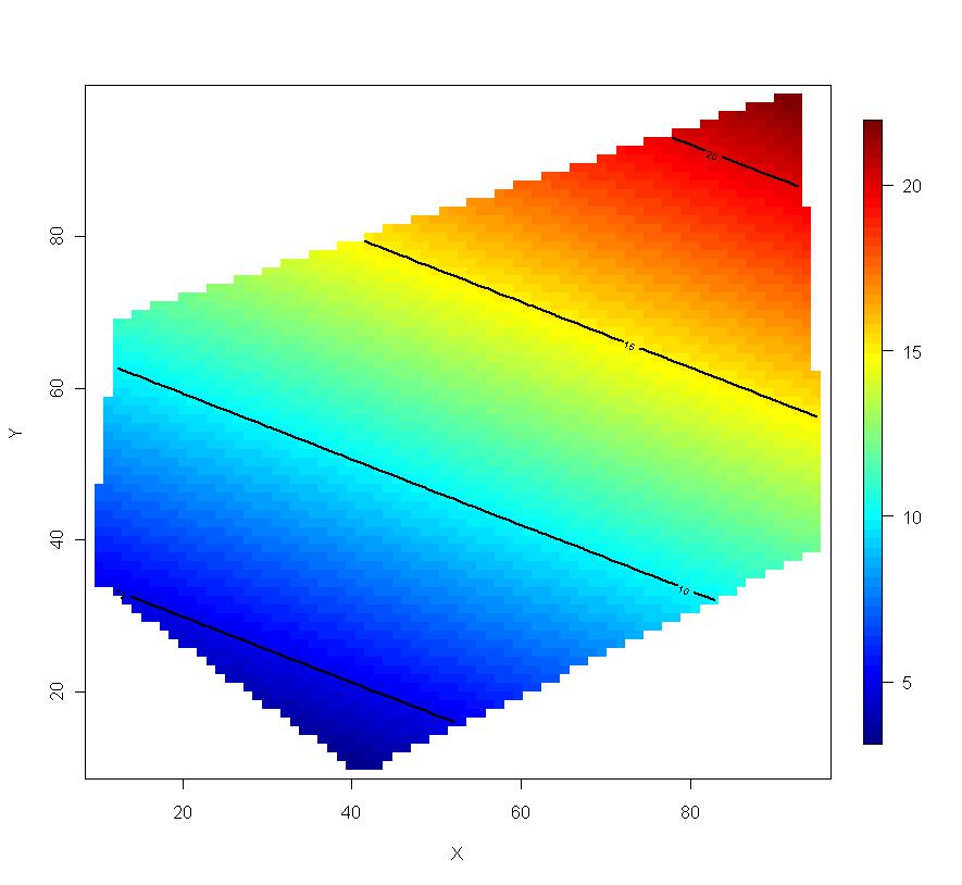
# Predict a grid
pred.grid = expand.grid(seq(0,100,l=51), seq(0,100,l=51)) # Define grid
# kriging calculations
kc = krige.conv(coord=cbind(X,Y),data=Z, loc=pred.grid, krige = krige.control(obj.m = ml))
image(kc, loc = pred.grid, col=gray(seq(1,0.1,l=30)))

# Using the "fields" library
library(fields)
fit = Krig(cbind(X,Y),Z,theta=95)
summary( fit) # summary of fit
set.panel( 2,2)
plot(fit) # four diagnostic plots of fit

set.panel()
surface( fit, type="C") # Display the surface